
Satellite Formation Flying for Space Advertising: From Technically Feasible to Economically Viable


1
Space Center, Skolkovo Institute of Science and Technology, 121205 Moscow, Russia
2
Moscow Institute of Physics and Technology (MIPT), 141701 Dolgoprudny, Russia
*
Author to whom correspondence should be addressed.
Aerospace 2022, 9(8), 419; https://doi.org/10.3390/aerospace9080419
Submission received: 30 June 2022
/
Revised: 27 July 2022
/
Accepted: 28 July 2022
/
Published: 1 August 2022
(This article belongs to the Special Issue Distributed Space Systems: Applications, Deployment and Control)
Abstract
:The paper presents a feasibility study of satellite formation-flying missions for space advertising. To estimate a space advertising mission viability, the global population coverage model is designed and the demonstration schedule with a focus on larger cities is optimized for the formation of small satellites deployed in repeat ground track Sun-synchronous orbits. Monetization of an image demonstration over a city depends on the city population, outdoor advertising cost, and parameters limiting the number of potential advertising observations. Formation lifetime expressed in terms of fuel consumption for image reconfigurations and maintenance is one of the key factors and is analyzed via numerical simulation of satellite formation-flying dynamics and control.
1. Introduction
Space advertising is a promising although still futuristic concept for outdoor advertising and the subject of arguments about rational and sustainable space exploration. The existing approaches for space advertising can be divided into single-time events and multiple demonstration event missions. There are examples of the former such as logos on board a rocket [1], branded food delivery to the International Space Station [2], or even a car launched to space [3]. However, in these examples, space advertising was merely a side-issue in a major space mission, whereas what we propose to consider is a dedicated space system. A long-term space advertising mission would rely on a complex satellite system orbiting the Earth and demonstrating pixel images to observers on the ground. In this case, an advertisement appears as a constellation of bright artificial stars formed into an image that can be observed in clear night sky for several minutes. Development of such missions has become a point of interest for a few space startups because the approach provides global Earth coverage and thus allows showing an advertisement to regions of high-demand multiple times [4,5]. Despite the fact that there are no successful examples of long-term space advertising missions, there were several attempts to launch them. First attempts were carried out in the last century. In 1989, to celebrate the Eiffel Tower centennial, it was planned to deploy a string of a hundred solar reflectors in the low-Earth orbit (LEO) to form a ring of light, visible throughout the world [6]. Another space advertising campaign was dedicated to the Olympics in Atlanta in 1996 [7]. The idea was to launch a big reflective sheet with a length of a mile and width of a quarter-mile that would be visible on Earth. Both missions, however, were to be devoted to a single event and relied on a space structure rather than on a satellite formation to display the graphics. The are two major options for producing space advertising in terms of a payload: solar reflectors and lasers. The former is used to reflect sunlight to a point of interest (POI) on Earth. It requires relatively large sunlight reflectors with an area of about 30 square meters [8] for LEO orbits to ensure the required pixel brightness as well as keeping the required reflectors’ attitude to illuminate the required region on Earth. The latter gives more flexibility on satellite attitude during image demonstration, but requires additional power supply.
Our prior studies have formed the concept of a formation-flying mission for long-term space advertising [8]. The proposed satellite formation comprises multiple CubeSats equipped with solar reflectors. Under certain geometrical conditions, each reflector can be observed from the ground as a bright star, and the group of satellites brought into a specific orbital configuration can be seen as a pixel image. The geometrical constraints or demonstration requirements define the lighting condition at POI and require all pixels within a demonstrated image to be clearly visible and distinguishable from each other. The lighting condition at POI is defined by the Sun elevation angle. We use the limiting value for the Sun elevation angle as the one that is used to define lighting conditions for astronomical observations [9]. Pixel visibility is expressed in terms of its apparent magnitude m and the minimum inter-pixel distance is defined by the angular resolution of a human eye that is known to be equal to about one arcmin. In [8], the mission design method for selecting target orbits for the mission, solar reflector sizing, and orbital configuration design were proposed. It was shown that the target orbits for the mission should be circular Sun-synchronous and lie close to the terminator plane. The type of orbits guarantees that formation satellites will always be lit by the Sun, and its access area will constantly include points on Earth where the lighting condition is satisfied. The orbital configuration of the formation is a set of projected circular orbits (PCO) defined with respect to the geometrical median of the image. The relative satellite trajectories are chosen in a way ensuring that all pixels are far enough from each other to be distinguished by a naked human eye during image demonstration above an arbitrary city for which the demonstration requirements are met.
The general logic for the satellite formation control applied for deploying, maintaining, and reconfiguring orbital configurations required for demonstrating multiple pixel images was proposed and an analysis of different types of relative motion control algorithms was performed. It was shown that the formation of solar-reflectors-equipped CubeSats can be controlled using aerodynamics drag-based control [10]. The propellantless approach allows deploying and reconfiguring the required orbital configuration within several hours if operating only at low orbits with altitudes below 400 km and using large enough solar reflectors which limits the formation lifetime. The hybrid control scheme comprised impulsive maneuvers for deployment and reconfiguration and a linear-quadratic regulator-based continuous control for reference orbits maintenance was proposed in [8]. The analytically derived impulsive maneuvers have smaller fuel consumption in comparison to the continuous one but have smaller precision and can be applied at a certain location on the orbit defined by the argument of latitude. Therefore, it must be complemented by the continuous control for relative orbits maintenance. In addition, depending on the formation orbital configuration’s linear size, the reconfiguration maneuvers may require relatively big thrust on the order of several N and greater, to apply the control impulse properly. This may require two different propulsion systems for reconfiguration and maintenance that is difficult to be integrated on-board a CubeSat. Therefore, in the study, the continuous LQR-based control algorithms requiring a single COTS thruster are applied for both reconfiguration and maintenance.
The study is devoted to the techno-economic analysis of long-term space advertising missions performed with the aid of formations comprised of solar reflectors-equipped small satellites. The following part of the paper is structured as follows. The second section introduces the main reference frames. In section three, the geocentric orbits that are used for the space advertising mission are derived. The fourth section is devoted to spacecraft payload—solar reflector and presents a method for its sizing. The fifth section discusses formation lifetime. It starts from an approach for the orbital configuration design used for an image demonstration mission, introduces relative motion control algorithms, and proposes methods for estimating satellite formation lifetime. In section six, the Earth coverage analysis is performed. Firstly, the coverage model is introduced. Secondly, the demonstration price model is presented. It assigns a price of an image demonstration to large world cities. Thirdly, the algorithm for calculating and optimizing Earth coverage and hence calculating and optimizing space advertising mission revenue is outlined. The study outcomes are reflected in the seventh section. The mission cost including mass production of formation satellites and their launch and services is estimated and compared to the mission revenue, to assess space advertising missions’ economic feasibility. The eighth section concludes the presented study.
2. Reference Frames
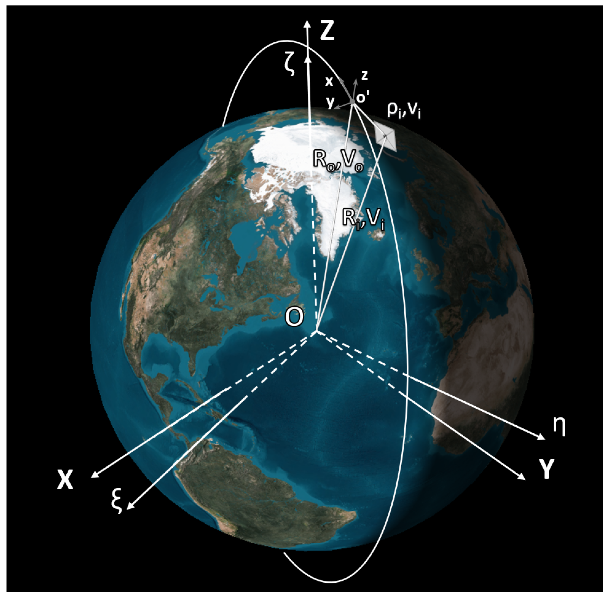
The reference frames used in the paper (see Figure 1) are as follows:
- The orthonormal basis is the Earth-centered inertial reference frame (ECI J2000) denoted by . ECI frame has its origin at the Earth’s center, its X-axis is pointed to the Sun at vernal equinox, Z-axis is aligned with the Earth’s rotation axis, Y-axis completes the reference frame to the right-hand triad.
- The orthonormal basis denoted by is the Earth-centered Earth-fixed reference frame (ECEF) which is a geocentric coordinate system fixed with the rotating Earth.
- The orthonormal basis is the orbital reference frame denoted by that has its origin at the target orbit, its z-axis is aligned with the local vertical, y-axis is directed along the target orbit angular momentum vector , and x-axis completes the reference frame to the right-hand triad.
The formation’s target orbit is determined by its state vector . The i-th satellite’s state vector given in is denoted by . The i-th satellite’s state vector given in is denoted by .
3. Target Orbit Selection
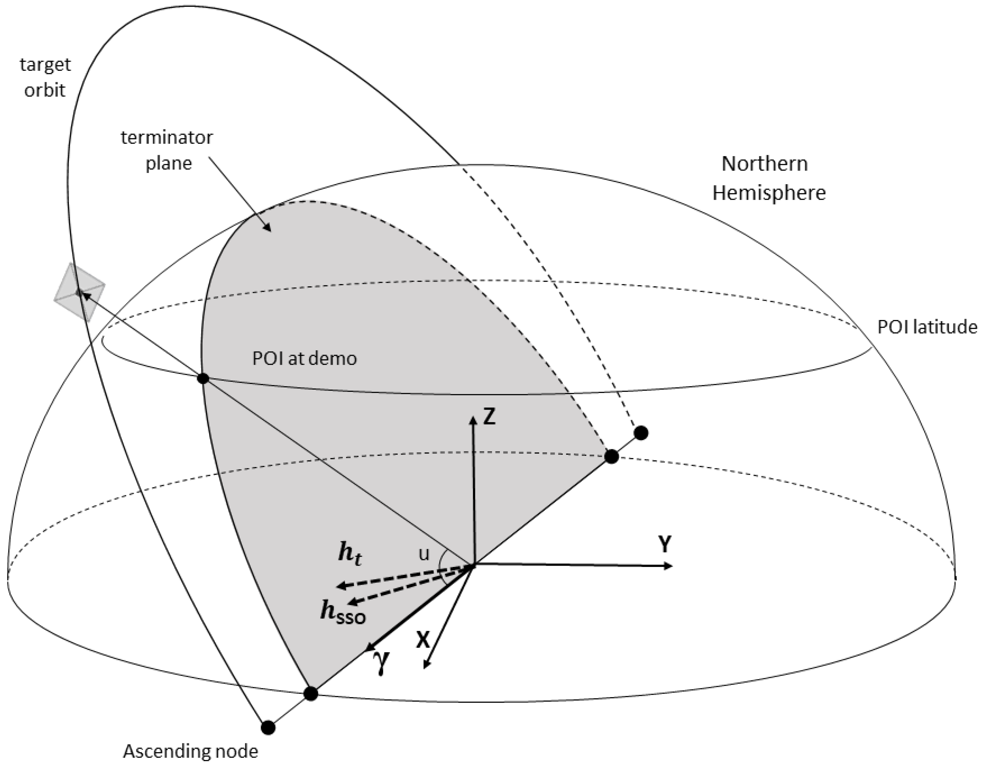
Following the conceptual mission design [8] for space advertising performed with the aid of solar sail-equipped formation-flying satellites, we consider near-circular Sun-synchronous orbits lying near the terminator plane. Satellites placed into such orbits are not only constantly illuminated by the Sun, but also have their POIs within satellites’ access area that have appropriate lighting conditions for image demonstration (). We shall employ the so-called repeat ground track orbits (RGT) which allow performing regular demonstrations at locations with high demonstration price, thereby increasing the mission profit.
The RAAN of the target orbit is chosen so that the orbital nodes belong to the intersection of the equatorial reference plane and the terminator plane. Given the unit orbital node vector , we obtain
The orientation of the orbit provides similar lighting conditions for morning and evening demonstrations. The orbital node vector can be determined from the normal to the terminator plane whose direction is chosen based on Sun declination and POI’s hemisphere as follows:
where is the unit vector (in ) of the Sun direction as seen from Earth, is a latitude of the target region. The orbit design geometry is illustrated by Figure 2, which shows the case for negative Sun declination and POIs location in the Northern Hemisphere.
Let us find an orbit with semi-major axis a and inclination i to make it Sun-synchronous with repeating ground track. For a Sun-synchronous orbit, the RAAN secular rate should equal the Earth mean motion around the Sun , where is the gravitational parameter of the Sun, and is semi-major axis of the Earth’s heliocentric orbit. The equation for a circular orbit RAAN precession rate [11] yields the orbit inclination i as follows:
where km is the mean equatorial radius of the Earth, n is the mean motion of the target orbit, is the radius of the target orbit, is second-order zonal harmonic of Earth potential.
For a repeat ground track orbit, the ratio between satellite nodal orbital period and nodal period of Greenwich meridian is the ratio of two integers [11]. Typically, the RGT orbits are defined by a number of satellite revolutions that should be made within days. For a Sun-synchronous repeating ground track orbit, the Greenwich nodal period is a fixed value defined as follows [11]:
where is the Earth self-rotation angular velocity.
The nodal period for circular orbits is given by [11]:
where is the Keplerian orbit period.
We shall consider the orbits that repeat daily to make image demonstrations over the most densely populated Earth regions as often as possible. The orbit altitudes range from 500 to 1000 km, because our prior research has shown that at lower orbits, the mission lifetime suffers from the excessive fuel expenditure to counteract the effects of the atmospheric drag, whereas the upper bound comes from the condition of having bright enough pixels while keeping the reflectors’ size to that which has been successfully operated in space missions. Given the altitude range, there remain two possible orbits to be used—the one that performs 15 revolutions per day and has 568.13 km altitude and another that performs 14 revolutions per days and has an altitude of 895.45 km. The latter is chosen to be the target orbit in the subsequent analysis, because it corresponds to the larger access area yielding greater mission revenue. The inclination of the 895.45 km altitude circular SSO is degrees.
4. Spacecraft Payload Sizing
Let us introduce the key parameters of a satellite for space advertising that are of importance for mission performance. These are the solar reflector’s area and the reflected light beam’s half angle .
Solar reflector parameters are used to set worst-case pixel magnitude during demonstration and reflected sunlight beam’s footprint area for a given satellite formation’s orbit. The pixel magnitude m relates to the reflected light intensity I at the observer locality as
where the reference intensity lux [12]. To calculate the reflected sunlight intensity at the observer location I, the following formula is used [13]:
where is the average intensity of the solar energy at a distance of 1AU (where the Earth is located), is the reflectivity coefficient, is the incident angle of solar rays, is the elevation angle of the satellite measured at POI, d is the distance between the reflector and POI, is the atmospheric transmissivity [13]:
Mylar film coated with aluminum is considered as the reflector material because of low weight and high reflectivity coefficient [13]. The reflector, which is deployed and maintained by a rigid support structure, is assumed to be of square shape (similar to previous solar sail projects [14,15]).
A procedure for solar reflector sizing is proposed in [8]. The idea is to find such an area of the reflector that satisfies the requirements to pixel brightness for the worst-case geometrical conditions during image demonstration. To this end, the minimum value of the intermediate parameter is obtained as:
The minimum value for the intermediate parameter can be used to relate the required intensity of the reflected sunlight at POI and solar reflector parameters— and using the expression:
Here and below, we study the system performance with the reference to the state of the art in solar reflector technologies to set the affordable reflector size for a CubeSat mission. According to [16], the largest solar sail size that have been successfully deployed and utilized on-board a CubeSat is 32 m. A flat reflector of that size produces a 54.6 km spot on Earth considering the 895.45 km orbit altitude and reflecting sunlight to sub-satellite point. Taking into account that most of world cities with large population usually have an area that is several times greater, we perform Earth coverage simulations for different footprint areas that can be achieved by using a paraboloid-shape diffusive reflector yielding a greater half beam angle but decreasing pixel brightness.
Let us consider the following geometrical approach to determine the relation between the pixel magnitude at the worst-case demonstration conditions and the solar reflector parameters for a specific mission. For this purpose, the critical values for parameters in Equation (10) are to be estimated.
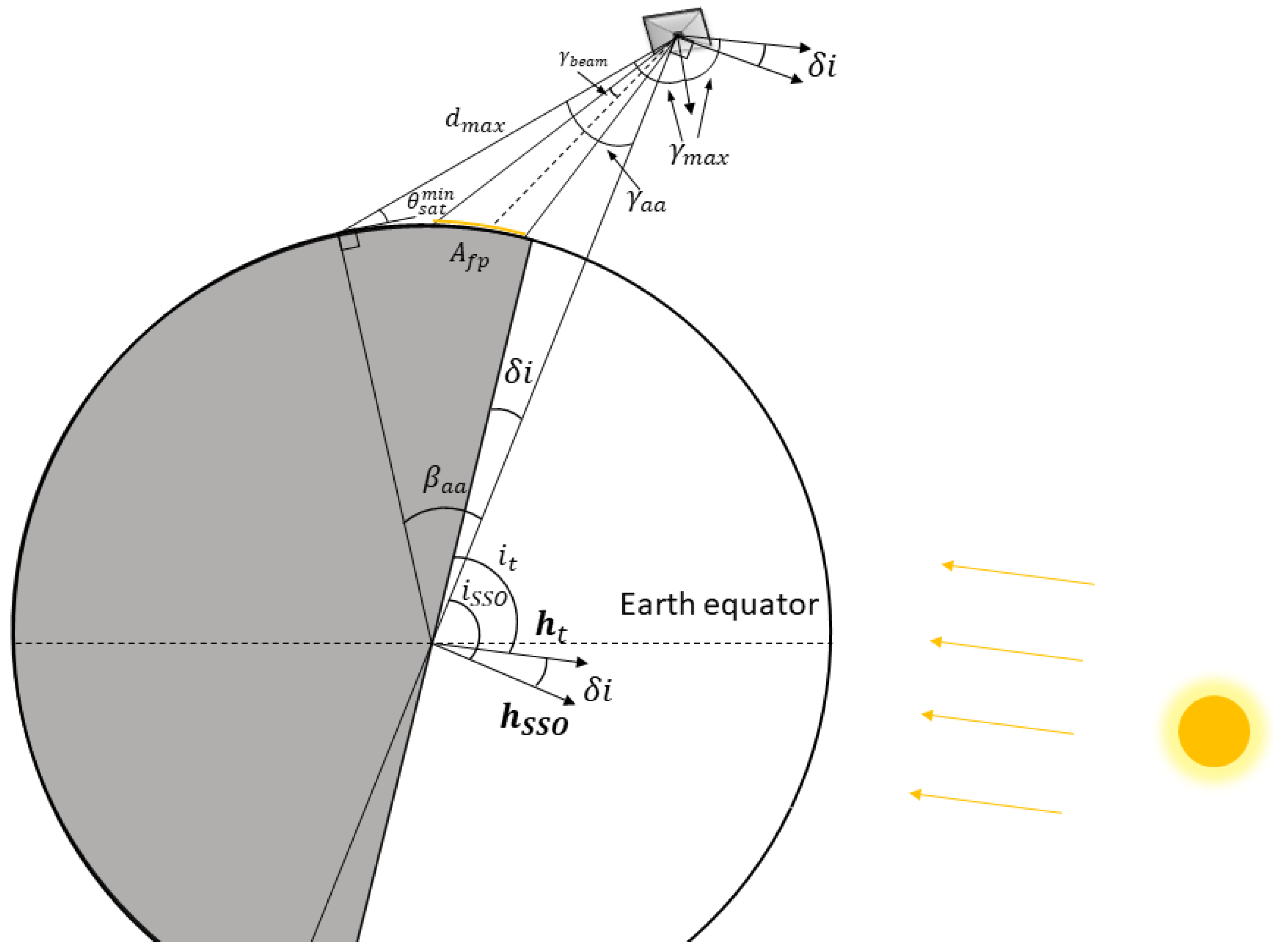
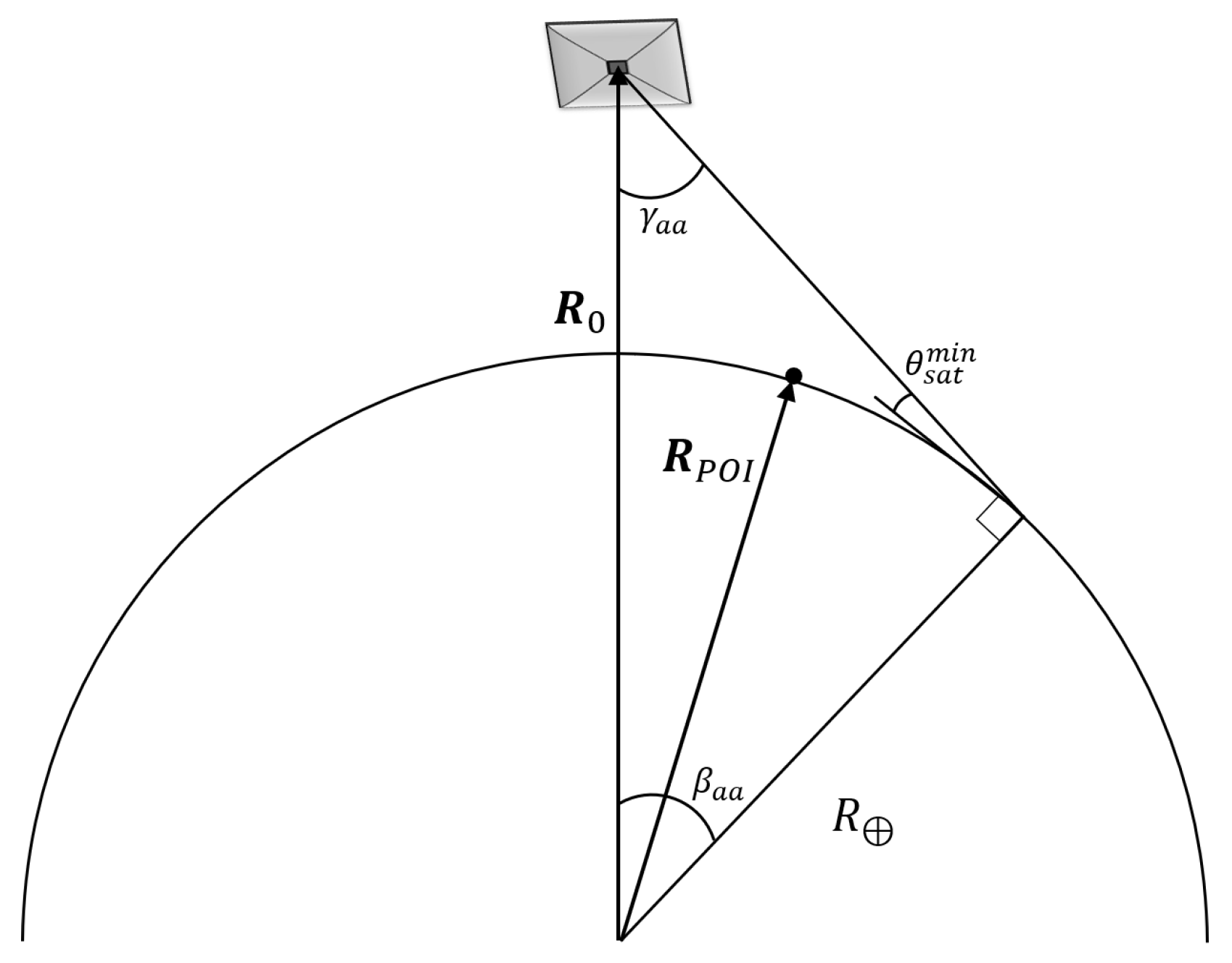
In order to make sure that all demonstrations scenarios satisfy mission requirements, we define worst-case conditions for all possible demonstrations events analytically. The task is to find the maximum distance to a POI during demonstration and the maximum sunlight incident angle . The minimum satellite elevation is set by image demonstration requirements and is equal to 10 degrees as in our previous study.
Let us consider the following geometry depicted in Figure 3.
The illustration portrays a mission geometry in a plane perpendicular to both terminator and orbital planes. From the sine law, the angle defining the satellite access area can be found as follows:
where , km is the mean radius of the Earth. The maximum sunlight incident angle can be found as
where , is the inclination of the terminator plane. The maximum possible distance between formation satellite and POI can be found using the cosine law as follows
where .
Given the half beam angle and orbit radius , the footprint area is calculated as follows:
The footprint area corresponds to the case when the satellite formation is located in zenith at POI and will be used to obtain a lower bound estimate for a demonstration mission revenue.
For the chosen orbit with an altitude of 895.45 km, the maximum distance to a POI is km considering minimum satellite elevation during demonstration . The maximum incident angle is which happens on summer or winter solstice.
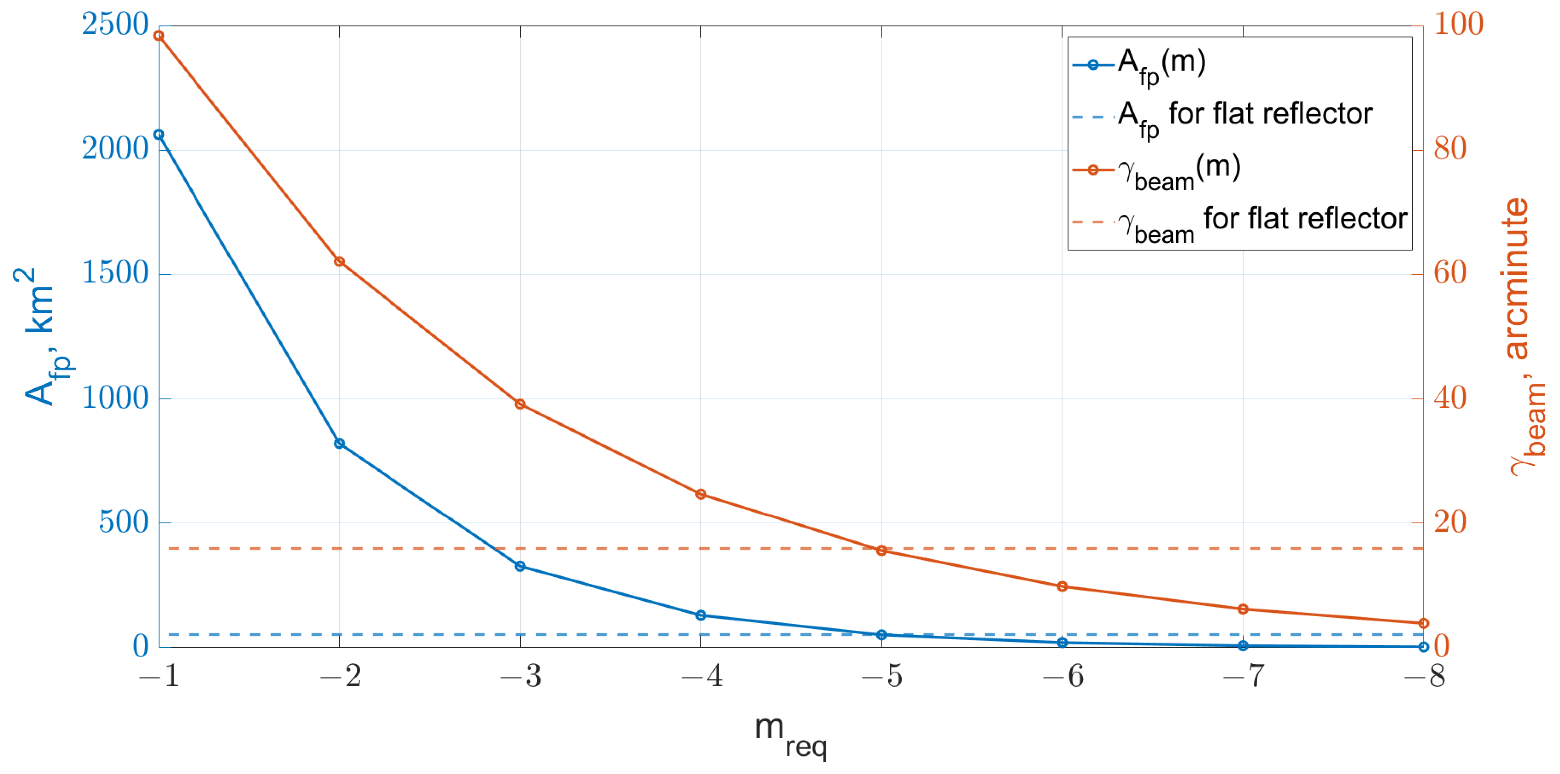
For the critical parameters, let us find the curve of the reflected half beam angle as function of the required pixel magnitude for a 32 square meter reflector. Figure 4 shows the dependence of the half beam angle on the required pixel magnitude ranging from −1 to −8 (blue line). The red line on the figure shows the corresponding footprint area. The horizontal lines represent the case of a flat reflector when its half beam angle is equal to the half angular size of the Sun known to be about .
The coverage simulations will be performed for the cases when footprint areas are similar or greater than the one of the flat reflector (see Table 1).
5. Formation Lifetime
5.1. Orbital Configuration
The considered space advertising approach is to display images constructed from a set of co-rotating pixels. The produced image has the same shape and size for observers at different locations on Earth while appearing at different orientations and slightly rotating during demonstrations of several minutes.
The orbital configuration for the satellite formation is a set of projected circular orbits (PCO). The PCO orbit is a type of periodic relative trajectories that can be found using general form of the analytical solution to the Hill–Clohessy–Wiltshire (HCW) equations describing relative motion dynamics between two satellites located at close circular orbits [17]. The HCW equations projected onto the orbital reference frame are the following:
where ,, are the components of i-th satellite position vector given in , is the control acceleration.
The periodic trajectory of an i-th satellite located at a PCO orbit is determined by two constants and corresponding to the radius of the trajectory’s circular projection onto the local horizontal plane and the phase angle in the projected circular orbit as given by:
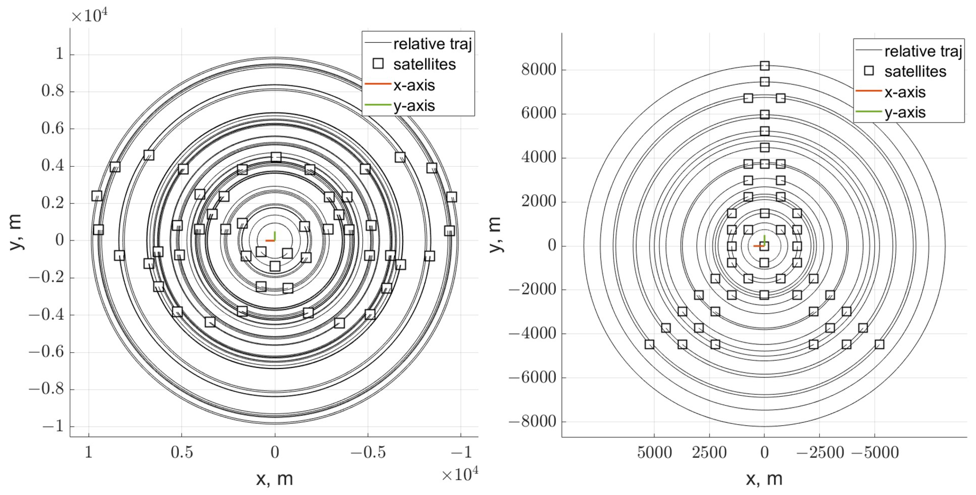
where phase . In order to define a set of reference trajectories with state vectors , for an image demonstration, polar coordinates of all image pixels must be found and used as constants and , and phase is used to define the whole image attitude with respect to the orbital frame. In this case, the image is seen as a set of co-rotating pixels visible in the sky as illustrated by Figure 5 portraying images borrowed from our prior study [8].
5.2. LQR-Based Continuous Control Algorithms
The LQR-based continuous-thrust control algorithms are used for satellite formation reconfiguration and maintenance. The control law is obtained for the linearized equations of satellite relative motion dynamics in the central gravity field to minimize the following objective function:
where is the satellite state vector deviation from the reference trajectory, and are the positive-definite diagonal weight matrices that determine the weight of errors for the state vector and the weight of the control resource consumption. The details on the LQR controller design can be found in [8]. The final formula for the control acceleration of the spacecraft (saturated according to the condition) is
where the optimal gain matrix
and is obtained from the algebraic Riccati equation given the weight matrices and , is the control matrix.
The controlled satellite dynamics is modeled in the ECI frame . The equation of orbital motion of i-th satellite is:
where is the control acceleration found according to (19) and transformed to the ECI frame, stands for external disturbance caused by the Earth oblateness given by [18]
where . All other perturbations are not considered. The orbital motion dynamics equations would normally include the influence of the atmospheric drag, which can significantly impact the orbit of satellites in lower orbits. However, as the target orbit is chosen to have the altitude of about 900 km (see Section 3), the drag force can be neglected.
In order to calculate fuel consumption and corresponding during maneuvering, the following equation is used:
where is the thrust force, is the gravitational acceleration at sea level, is the specific impulse of the thruster.
Let us note that the proposed orbital motion dynamics model (20) omits the satellite state estimation error which contributes to the accuracy of the controller input. The control error in real-life missions is estimated from the sensors’ measurements, which may be additionally processed by an algorithm to reduce the measurement and process noise. The position and velocity of a spacecraft is usually determined by a GPS-receiver, and the relative positions of spacecraft in a formation-flying mission can be enhanced with the aid of the Differential GPS technique [19]. For example, The Radio Aurora eXplorer (RAX) CubeSat mission [20] launched two CubeSats containing a GPS subsystem. The position accuracy (standard deviation errors) was found to have a mean of 2.89 m and a maximum of 4.02 m. The CanX 4&5 mission [21] with similar or worse position accuracy has demonstrated a relative position control with a sub-meter accuracy. Recent developments of DGPS [22] show the promise of providing nanosatellite-based distributed space systems with centimeter-level relative position accuracy. The state estimation accuracy and corresponding control errors demonstrated in the aforementioned missions are within the image demonstration mission requirements, determined by what can be observed as a misalignment of the formation’s geometry by a human eye. Therefore, taking into account that our simulations aim mainly at estimating the formation lifetime, we shall confine ourselves to the consideration of an ideal position and velocity signals and neglect the measurement noise in all subsequent simulations.
5.2.1. LQR Gains Optimization for Reconfiguration
As shown in [8], the reconfiguration maneuvers play a major role in fuel consumption. Therefore, we propose a procedure for LQR weight matrices , tuning based on a multi-objective genetic algorithm to improve the system performance. The gain matrices thus tuned are applied during reconfigurations.
The space advertising application poses stringent requirements to the relative motion control algorithms. On the one hand, the application requires relatively fast reconfiguration of the formation’s orbital configuration in order to change advertising image for demonstrations at different Earth regions. On the other hand, the distributed system should operate for a relatively long time on the order of several months to be economically feasible. Thus, the key performance metrics of the control algorithms for the considered application are the reconfiguration time and fuel consumption F. The reconfiguration time is the time it takes a satellite to reach the vicinity of a reference trajectory such that , starting at a given relative trajectory.
The bi-objective optimization is applied to minimize both fuel consumption for reconfiguration F and reconfiguration time . The optimization problem is stated as follows:
where and are components of the weight matrix such that
It is assumed that the weight matrix satisfies . We perform multi-objective optimization of control gains using an open-source framework for multi-objective optimization in Python [23]. The Non-dominated Sorting Genetic Algorithm (NSGA-II) is applied.
5.3. Assignment Problem
Satellite formation reconfiguration starts when the spacecraft is located at relative trajectories denoted by and has a goal to deploy a required orbital configuration defined by a set of reference trajectories . Taking into account multiple locations for graphics demonstrations and the fact that the projected images constantly rotate with respect to the orbital reference frame, it is inevitable that the images are observed in different orientations at different Earth regions. On the other hand, the reconfiguration fuel consumption depends on the relative image’s orientation that is defined by the phase . Therefore, we propose to optimize the orientation of the image to be deployed with respect to the initial state of the system, which should lead to the optimized fuel consumption.
Let us introduce a reconfiguration cost-matrix whose elements are
and represent the Euclidean distance between the current position of the i-th spacecraft and the j-th slot in the new configuration the formation should converge to. Given the cost matrix , we can formulate and solve the assignment problem [24] which assigns each satellite to its position in the new configuration such that the sum of distances that all spacecraft travel during the reconfiguration is minimized. Let us note that the solution to this problem not only determines the spacecraft positions in the new configuration, but also fixes the value of the phase parameter as
The exact optimization problem statement is then as follows. Given two sets of equal size : spacecraft (workers) and reference trajectories (tasks) and also the weight function , find the value of and a bijection such that the cost function
is minimized.
The proposed method allows choosing proper image’s relative orientation to minimize fuel consumption without actually computing the fuel consumed for transfers between current relative trajectory to that turns out to be a computationally intensive problem subject to the dimensionality curse. Finally, the assignment problem is solved for the set of reference trajectories using the cost matrix
that represents the costs of transfers of a to a new in terms of the consumed fuel. To build the cost matrix , the controlled satellite dynamics is simulated according to (20). The assignment problem that minimizes the total amount of fuel summed over formation spacecraft is solved [24].
5.4. Formation Lifetime Estimates
Let us estimate the mission lifetime for the chosen target orbit and the orbital configurations presented in Figure 5. The estimate can be derived from the mean fuel consumption for reconfiguration between orbital configurations and mean monthly fuel consumption for reference orbits maintenance. We shall assume that the reconfiguration is what takes place after the cluster launch when the formation needs to be deployed into an image or whenever there is a need to change the orbital configuration and start displaying a new image. At all other times, the formation spacecraft operates in the maintenance regime.
In order to calculate the mean fuel consumption for reconfiguration, let us optimize LQR gain matrices as described in Section 5.2.1. The initial deployment is the most costly maneuver in terms of fuel consumption, especially for the reference trajectories that lie farther away from . Therefore, we apply LQR weight matrix coefficients and optimization procedure for the transfers to the reference trajectory with the greatest radius of the projected circular orbit m. All simulation parameters with their values are listed in Table 2.
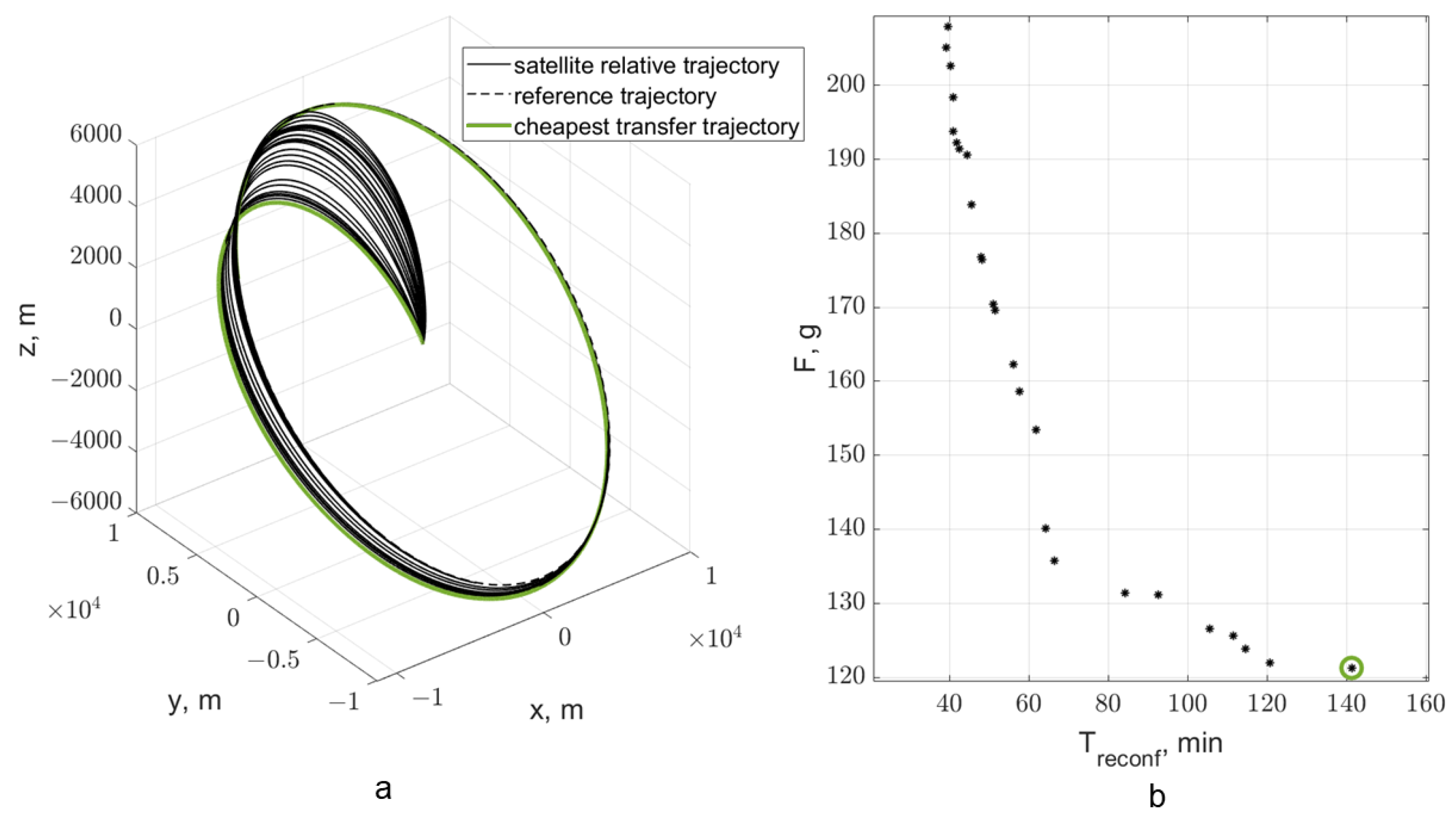
Figure 6a shows transfer trajectories to the farthest reference orbit for different sets of and corresponding to the Pareto front shown in Figure 6b.
Let us further use the LQR gain matrix corresponding to the solution marked by the green circle in the Pareto front (see Figure 6b) for the reconfiguration fuel consumption estimates. It corresponds to and . The gain matrix corresponding to the chosen and weight matrices can be seen in Appendix A.
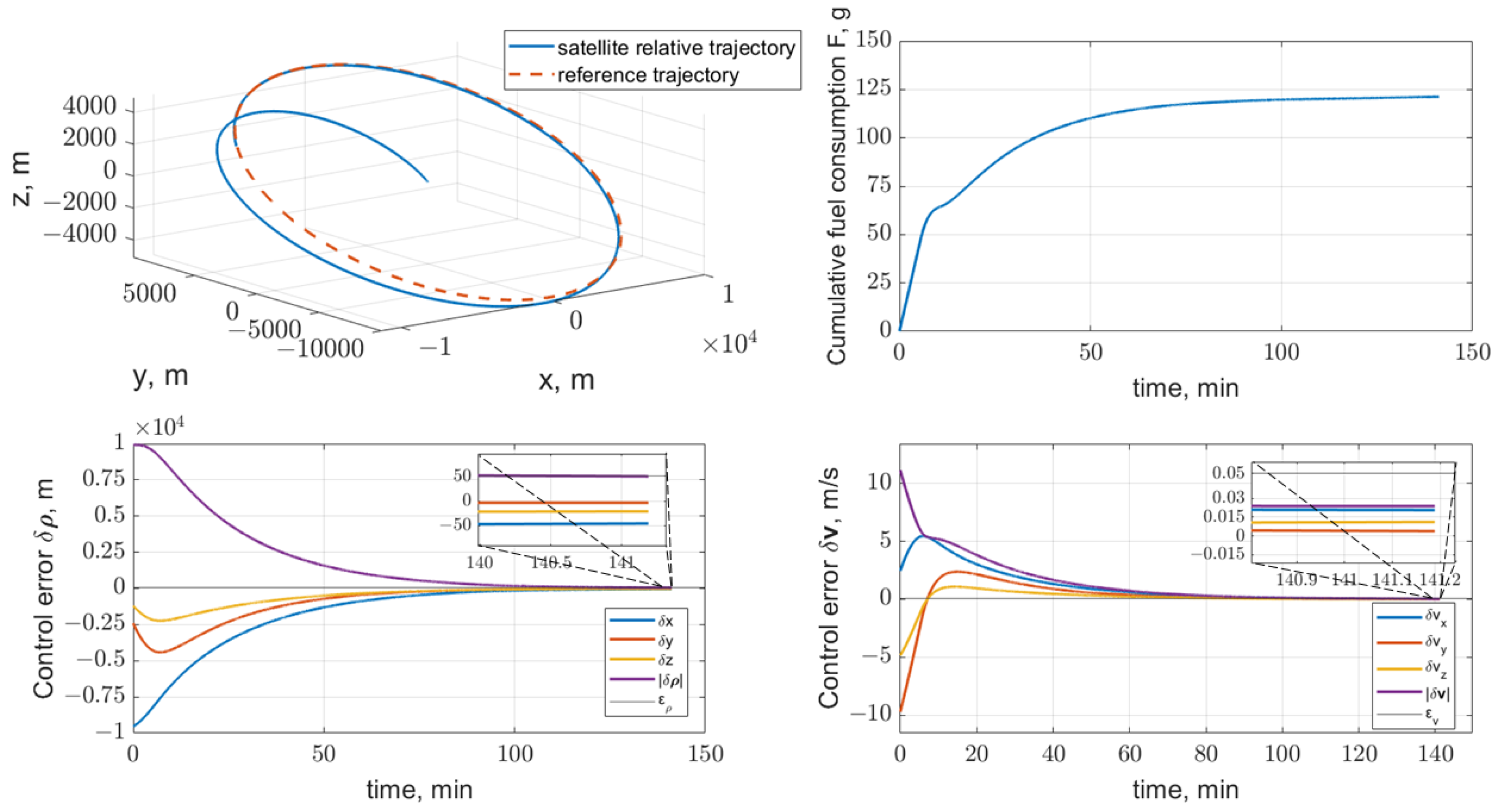
Figure 7 demonstrates the control algorithm performance for the chosen gain matrix . Top left graph represents the relative satellite trajectory during deployment, top right shows cumulative fuel consumption, and bottom graphs depict the control errors and during deployment. It takes 141 min and 121.3 g for reaching the reference trajectory.
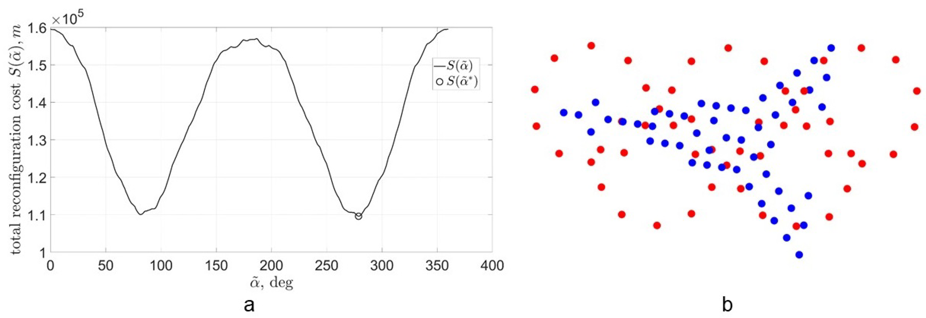
Let us now estimate the mean fuel consumption for reconfiguration between the two orbital configurations using the obtained gain matrix . As a first step the assignment, problem for different relative images’ orientations characterized by is solved using cost matrices to find the lowest reconfiguration cost and corresponding image phase (see Figure 8a). The procedure is performed according the approach proposed in Section 5.3.
Figure 8b shows the image’s relative orientation yielding the cheapest reconfiguration cost according to the chosen metric.
For the set of reference trajectories , the cost matrix is obtained via numerical simulation of the controlled dynamics of i-th spacecraft transferring to j-th reference trajectory. The assignment problem is solved for the cost matrix yielding the smallest sum of fuel consumption of formation satellites.
Figure 9a shows formation satellites’ fuel consumption for reconfiguration and reconfiguration duration for the obtained reconfiguration scenario from the assignment problem. The maximum fuel consumption during reconfiguration is 92 g while the mean fuel consumption is g.
In order to estimate monthly fuel consumption for reference orbit maintenance, the controlled satellite dynamics is simulated for all formation satellites assigned to the set of reference trajectories . For this purpose, the LQR gain matrix is used corresponding to the , and (see Appendix B).
Figure 9b shows monthly fuel consumption for maintenance of i-th reference trajectory. It can be seen that the mean monthly fuel consumption for maintenance is g.
Finally, the formation which has to perform reconfigurations per month has an estimated lifetime of:
Figure 10 represents the formation lifetime for different number of reconfigurations per month for the obtained mean reconfiguration cost and mean maintenance cost for different propellant masses .
6. Earth Coverage
This section is devoted to the Earth coverage analysis. Let us recall that the mission is about reflecting sunlight onto the Earth surface and the objects of interest to be covered by the resulting beams are large cities. The Earth coverage is calculated to estimate the revenue of a space advertising mission and the obtained estimates are later used to assess the economic feasibility of space advertising.
6.1. Coverage Model
Figure 11 presents the classical geometrical considerations used in Earth coverage models. All vectors are given in their representations in the frame. The state of the origin of the frame moving along the target orbit is . An i-th city’s position vector corresponds to the position of the city’s center given in . The data on locations, areas, and population of world cities are obtained from [26].
Let us assume that an i-th city is a potential location for an image demonstration if it lies within the formation’s access area and has proper illumination conditions. The access area is expressed through the angle . It is the maximum angle between the orbital reference frame origin’s position vector and the position vector of an i-th city when the city can be covered or an observer can see the projected image taking into account the requirement on the minimum satellite elevation angle during demonstration.
Finally, the cities where the image demonstration can be performed at certain moment are those for which the following conditions are satisfied:
where and are unit vectors of orbital reference frame’s origin and an i-th city position vector given in , is the Sun elevation at i-th city.
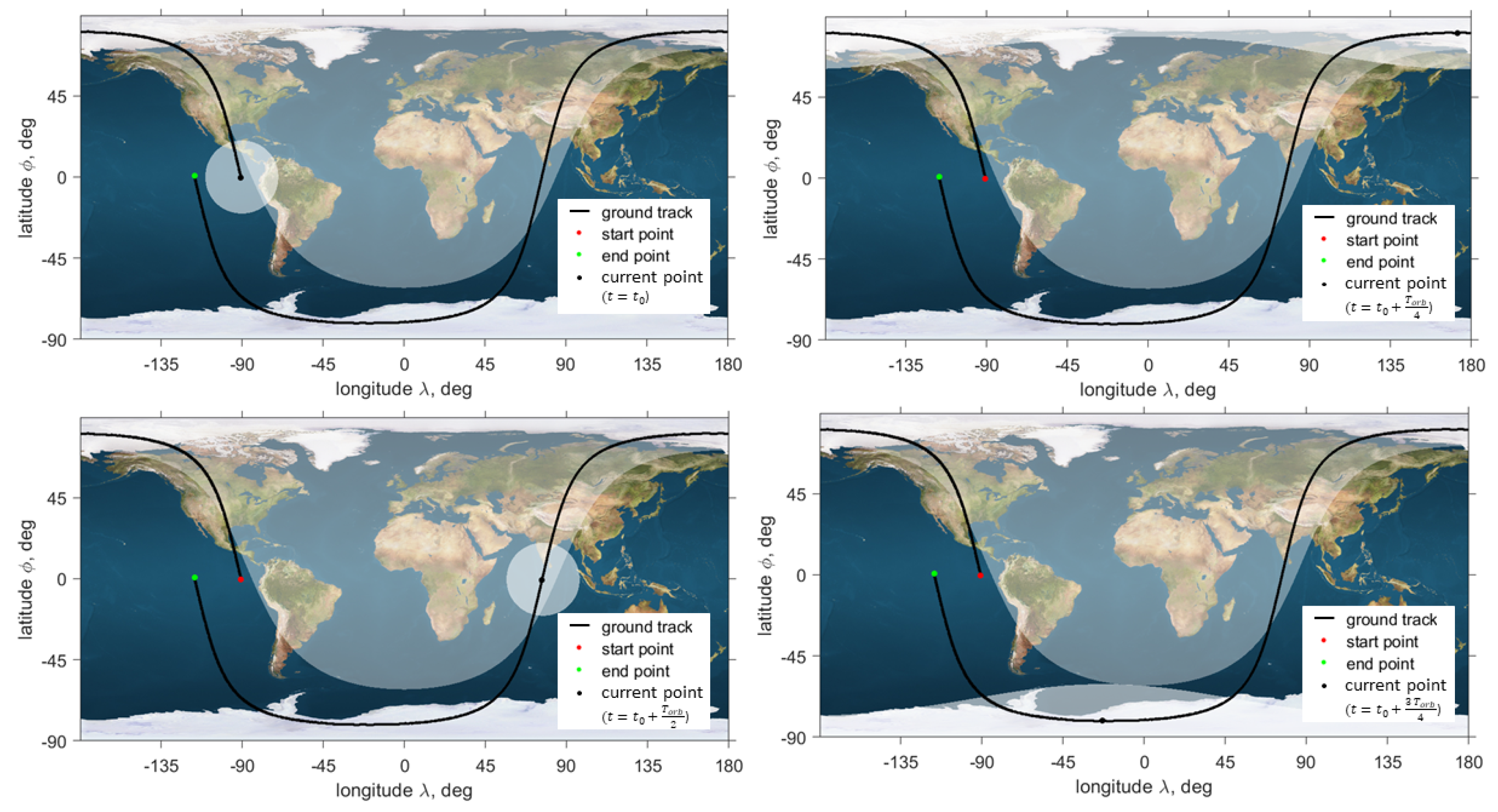
Figure 12 illustrates the proposed coverage model. It shows the ground track of the chosen Sun-synchronous repeat ground track orbit for one orbit period and formation’s access area and the region on Earth where the lighting condition is fulfilled for different time moments split by the quarter of the orbit period. The demonstration can be performed at cities located in the intersection of the highlighted regions.
6.2. Demonstration Price
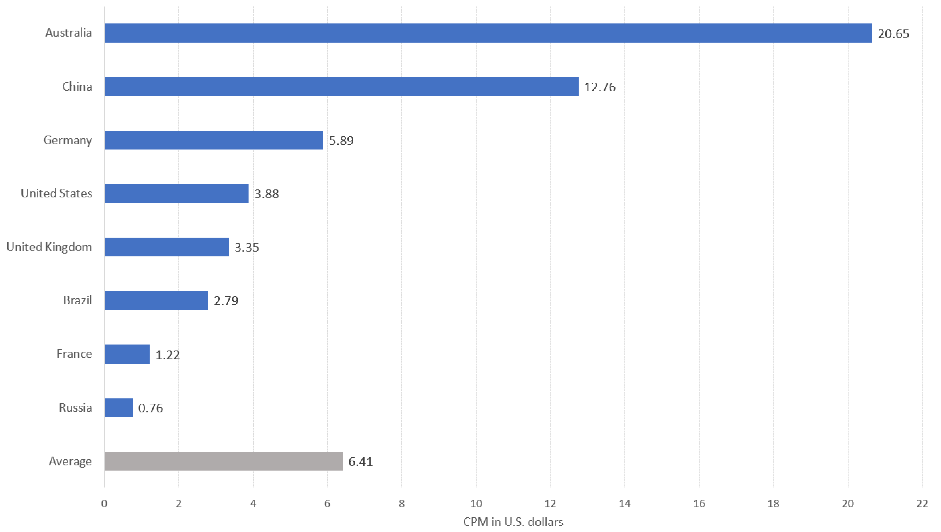
To assess the economic feasibility of a space advertising mission, we shall estimate price per single view in terms of CPM (Cost-per-mille), i.e., the price of a thousand ad views. There are various approaches to measure CPMs depending on the advertising campaign scenarios; however, in this study, we shall assume that space advertising CPM values are similar to those for large format billboards. The country-wise CPM values that we shall use are based on the open source statistics [27], which is collected for 2018, and remains qualitatively the same since then [28]. The average CPM for major countries in 2018 [27] are shown in Figure 13.
The amount of funds that can potentially be obtained from the demonstration in an i-th city is defined by how many views the advertising collects, which is the product of price per single view and the number of potential viewers in i-th city. Thus, we need to estimate the fraction of the population that can watch the demonstration at a certain point and at a particular time, because outdoor advertising cannot reach 100 percent of the population. This shall be expressed by the so-called opportunity-to-see (OTS) coefficient, which rates the number of exposures of a particular audience to a specific advertisement.
The expression for where subscript i denotes a particular city is:
where , , are discounting coefficients (whose values range from 0 to 1) that represent the influence of external factors such as seasonal difference, cloud interference, and demographic distribution, respectively. The values of discounting coefficients can vary over time.
Let us describe the discounting coefficients in greater detail:
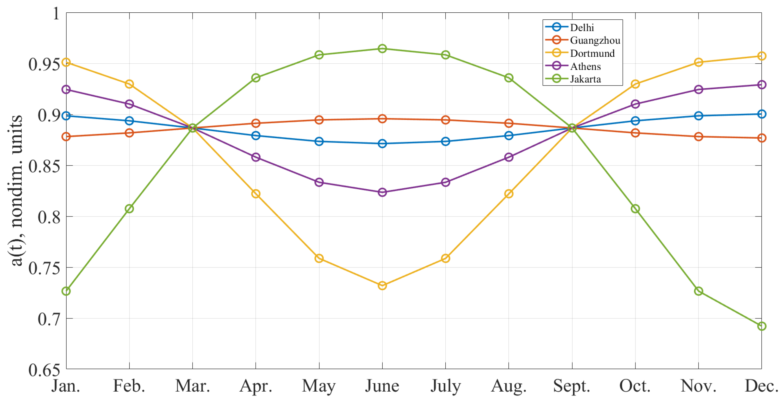
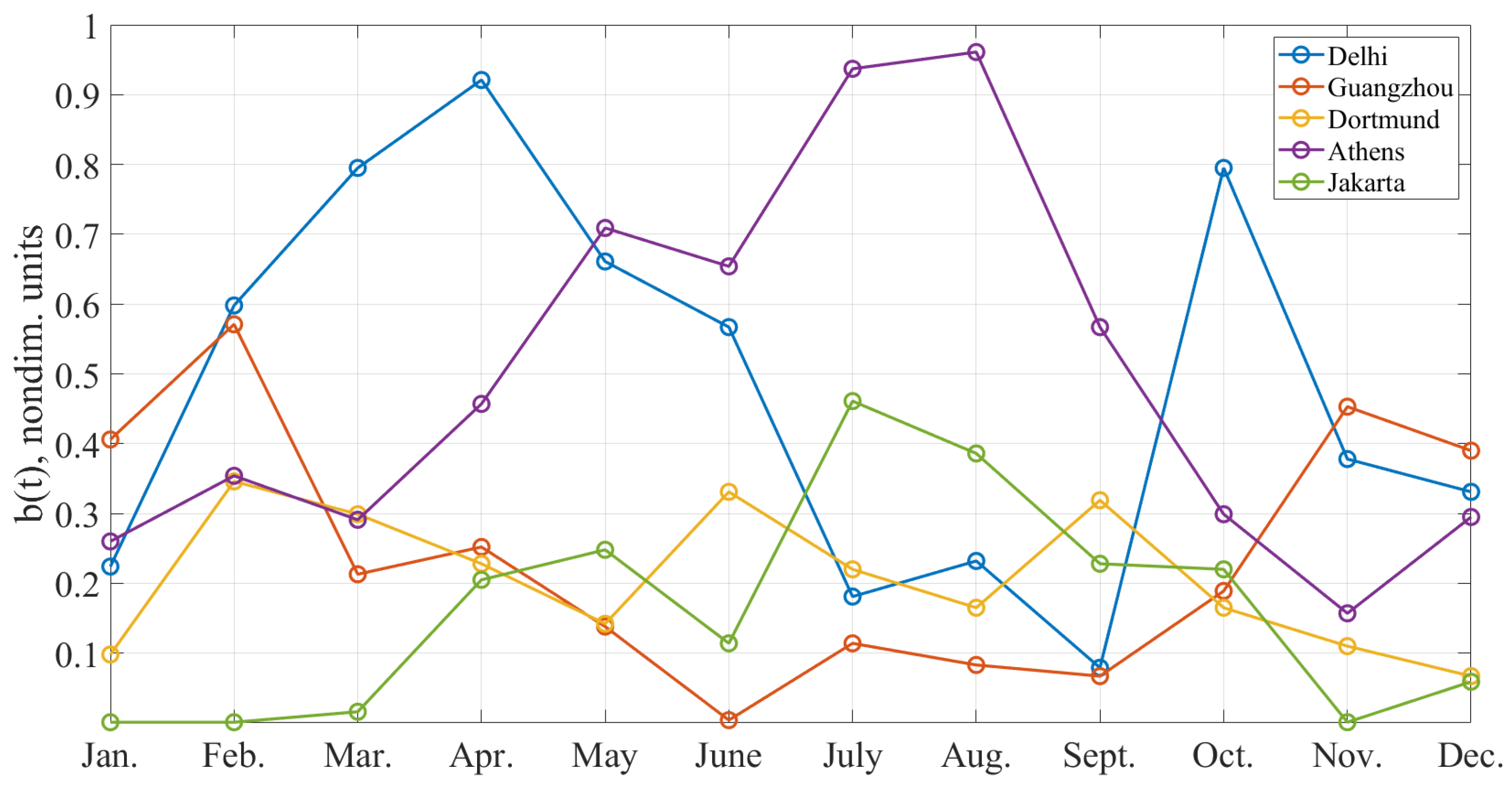
- The seasonal coefficient. The total number of the so-called impressions (i.e., contacts with the advertisement) varies significantly with the season change. For example, the probability of observing an outdoor demonstration during the calendar winter reduces owing to weather conditions. Therefore, it is necessary to take into account the month in which the space advertising demonstration takes place as well as the POI’s distance to the tropical belt. Areas located close to the tropical zones have mild and comfortable climate, which contributes to the frequent presence of advertising consumers outdoors. It leads to an increase of probability of the demonstration to be noticed. In these areas, the weather differences are not pronounced by seasons. At the same time, the visibility depends on the level of natural light: the lower it is, the less a person’s attention is scattered (people become more determined on the choice of the road). The overall level of illumination depends on the average length of the day, which, in turn, has an annual cycle and is expressed by the cosine function. The maximum of this function can be considered June, the minimum is December in the Northern hemisphere.The formula that takes into account the influence of the month of observation and the location of the object with respect to the tropical zones was obtained in [29]. The expression for the seasonal coefficient a for the city at latitude is given by:where and are the statistical coefficients [29], is the absolute value of tropic latitude (coincides with the latitude of Tropic of Cancer in the Northern hemisphere and with the latitude of Tropic of Capricorn in the Southern hemisphere), is the month of demonstration (from 1 to 12). Figure 14 illustrates the change of the seasonal coefficient over a year, for a list of cities with the greatest demonstration price at different Earth regions.
- The cloud interference coefficient.The cloud interference is expressed as the part of the Earth’s surface covered by clouds, relative to the part of the Earth not covered by clouds. The data on the cloud interference are taken from the MODIS Cloud Product [30]. These data represent the monthly values of the cloud fraction averaged from cloud groupings of 5 km × 5 km in size with maximum pixel resolution. These values are approximations based upon the scaled range of satellite images. The cloud fraction value for a specific i-th city is denoted by . To estimate the coefficients, data for different months of 2021 are taken from [30]. Thus, for each city, the coefficient representing the cloud fraction above city is varying depending on the month defined. Figure 15 illustrates the evolution of the cloud interference coefficient within a year for a list of cities with the greatest demonstration price at different Earth regions.
- The demographic coefficient. Individual differences between message recipients can lead to discrepancies in how people respond to advertisements. Thus, taking into account the characteristics of the population parameters allows constructing a more realistic model of economic viability for advertising missions. Residents older than 15 years are considered to be the solvent audience; thus, our statistics take into account people aged 15 years and older. The audience is divided into 3 age groups: 15–24, 25–64, 65+.The approach to describe how people of different age respond to outdoor advertising is described in [29]. The overall response is expressed as a weighted sum of age-group fractions, with weights selected to approximate the statistical survey data [31]. The expression for the demographic coefficient c (determined for each country) has the form:where and are the linear regression coefficients [29], whereas , , are the fractions of population that belong to the age categories denoted by the subscripts. The demographic parameter is determined on the scale of the countries; thus, it has the same value for all cities that belong to the same country.
Let us note that the cities with a population greater than ( = 50,000) are considered due to the economic impracticality of space advertising in sparsely populated locations. Coordinates of the cities and their population are in accordance with the Atlas of the Human Planet [26]. Each city with the is associated with a set of coefficients (, , ), where and vary depending on the month and is constant. Finally, the price of demonstration in i-th city is given by:
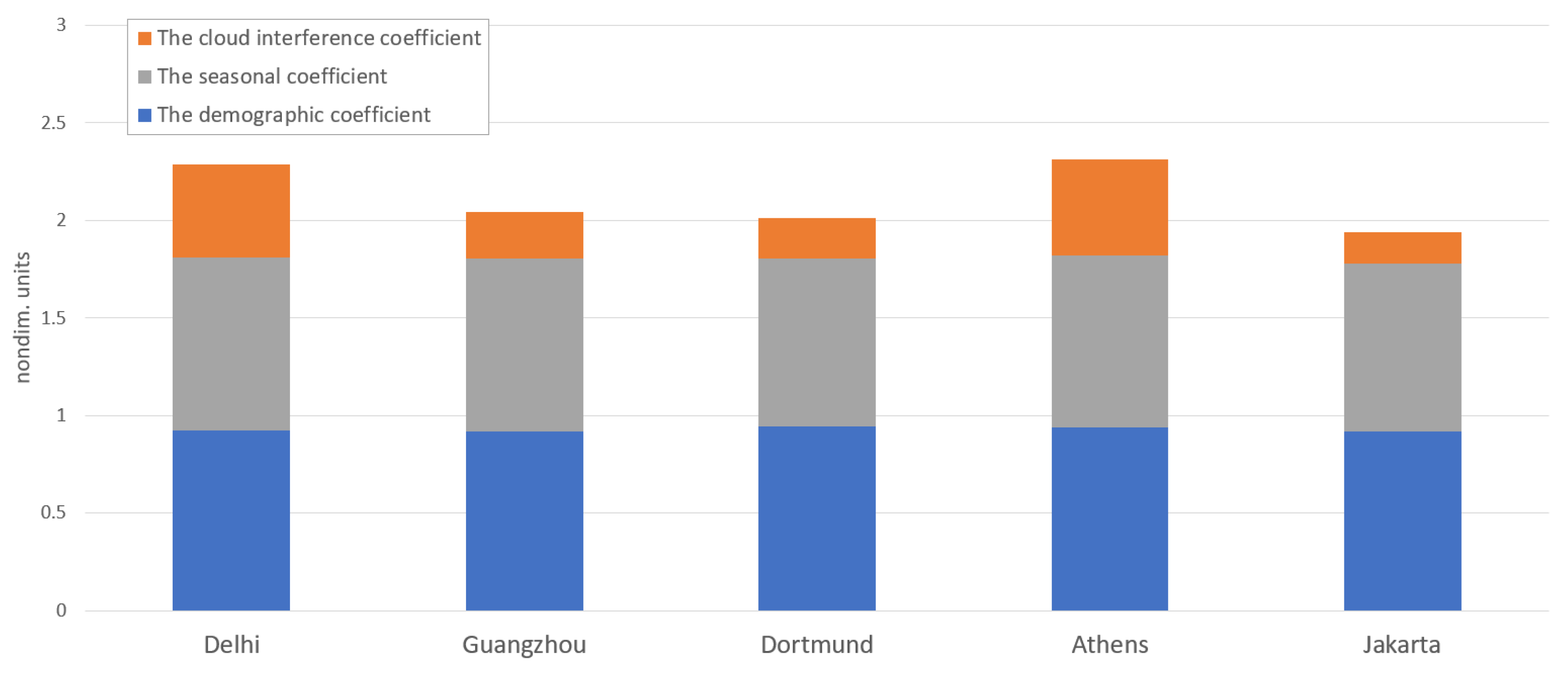
Let us note that the demographic and average seasonal coefficients , are not so sensitive to the location as the average cloud interference coefficient . The bar chart on Figure 16 shows the values of the three coefficients for the same list of cities as in Figure 14 and Figure 15 averaged over 12 months.
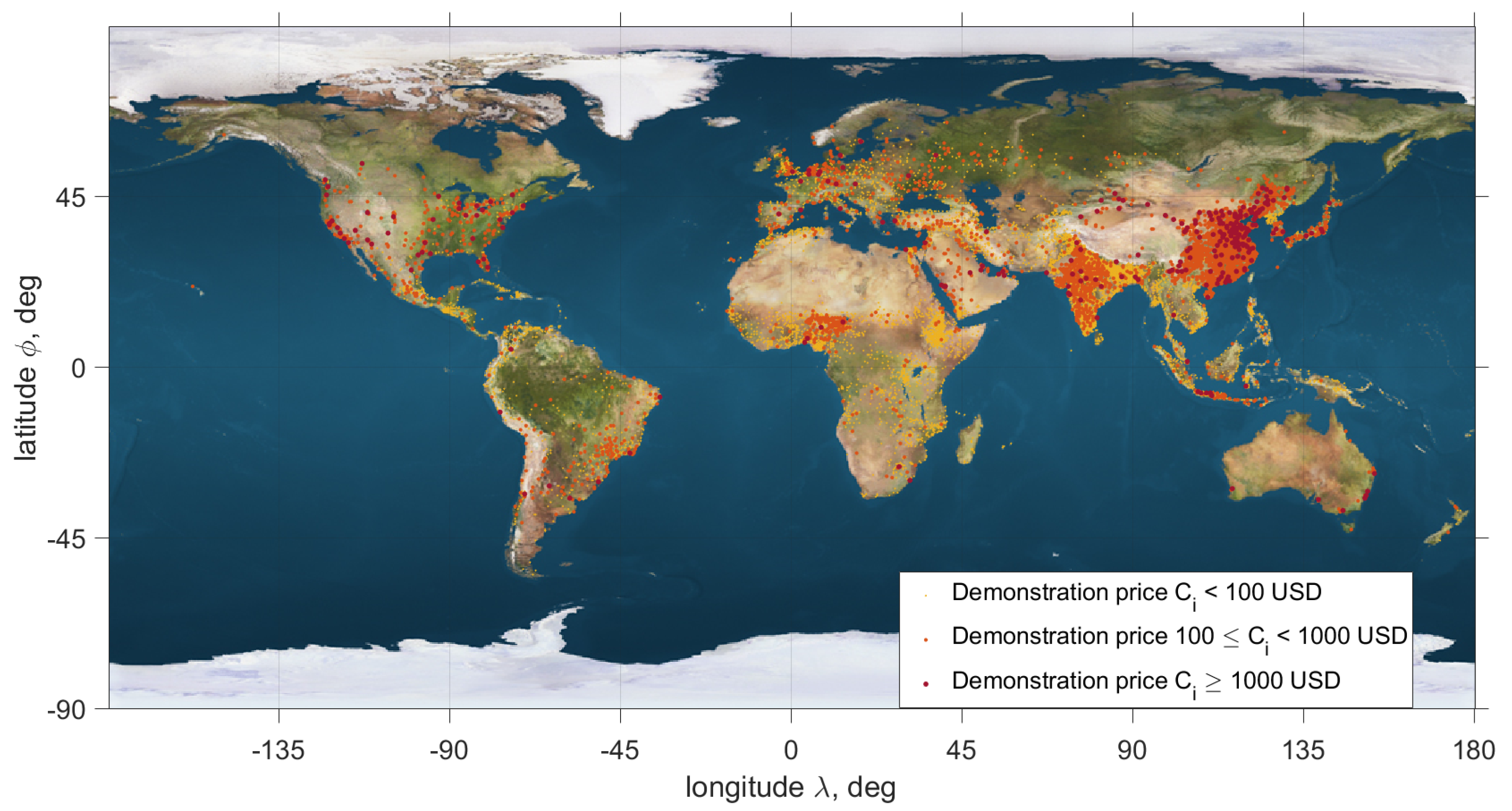
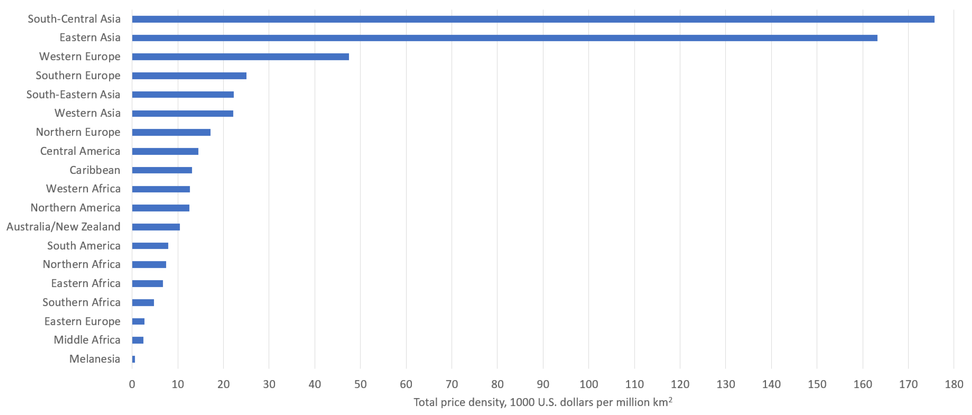
The world demonstration price chart is presented in Figure 17. The graph shows the mean (averaged over 12 months) values of demonstrations prices. The figure represents the most important regions where image demonstration brings more benefit. It can be seen that the most profitable regions are Western Europe, South-Central and Eastern Asia. The regional demonstration price densities corresponding to the average values of discounting coefficients , are presented in Figure 18.
The demonstration price distribution is of considerable importance in selecting formation’s target orbit. The idea is two find such an orbit that will allow to cover as much cities with a high demonstration price as possible during the mission.
6.3. Coverage Calculation and Optimization
To estimate the revenue of a space advertising mission, the Earth coverage is calculated for one day—the time it takes the ground track to repeat for the considered target orbit. Let us consider demonstration mission with fixed demonstration duration s and time between demonstrations that can be used for solar reflectors re-orientations s.
Let us note that the mission admits different demonstration strategies. For example, a strategy could be aimed to perform image demonstrations with the maximum duration limited by geometrical constraints (24). Nevertheless, the strategies assuming short demonstrations allow covering a greater number of cities and, hence, an increase in mission revenue.
Let us note that the region on Earth for which the demonstration conditions (24) are met can include multiple cities. Therefore, choosing different cities where demonstrations are to take place will influence the mission revenue.
To design a demonstration schedule or a sequence of cities with corresponding time when a demonstration is to be made, the target orbit dynamics is simulated according to (20) for each time step a list of cities is composed where the image demonstration requirements (24) are satisfied. A city within the list with the greatest demonstration price is selected for the demonstration and added to the demonstration schedule.
Let us note that the demonstration prices introduced in Section 6.2 correspond to the case when the whole territory of a city is covered. Therefore, taking into account that a satellite typically has a smaller footprint area , let us redefine the demonstration price for a specific demonstration mission as follows:
A city can be a location for image demonstration if the time period for which the demonstration conditions (24) are satisfied is not shorter than the pre-defined demonstration duration . In addition, if an i-th city is added to the demonstration schedule, it cannot be a location for the image demonstration for at least one orbit period.
The total price of demonstrations for a mission with image demonstrations is then defined as follows:
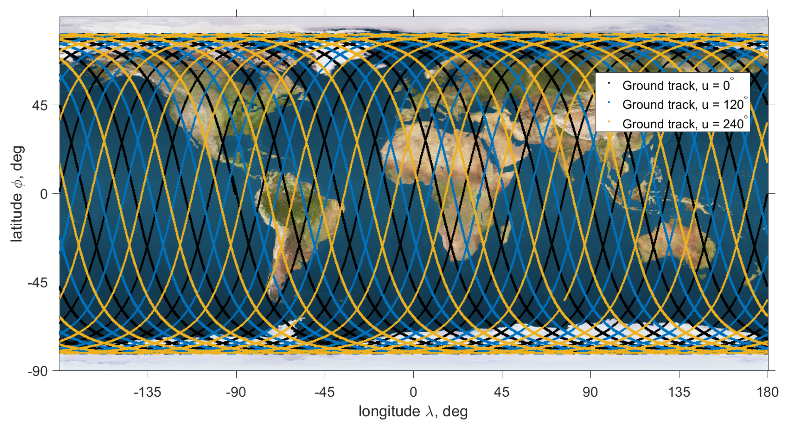
The demonstration revenue depends on the target orbit’s ground track that can be adjusted by the argument of latitude of the target orbit u for the fixed orbit epoch. The ground track is a set of elevation angle and azimuth angle of the orbital reference frame origin position vector given in the noninertial frame . Figure 19 illustrates the change of the orbit ground track depending on the argument of latitude u with the initial conditions presented in Table 3.
To optimize the demonstration revenue, the following optimization problem is solved using the Nelder–Mead algorithm [33]:
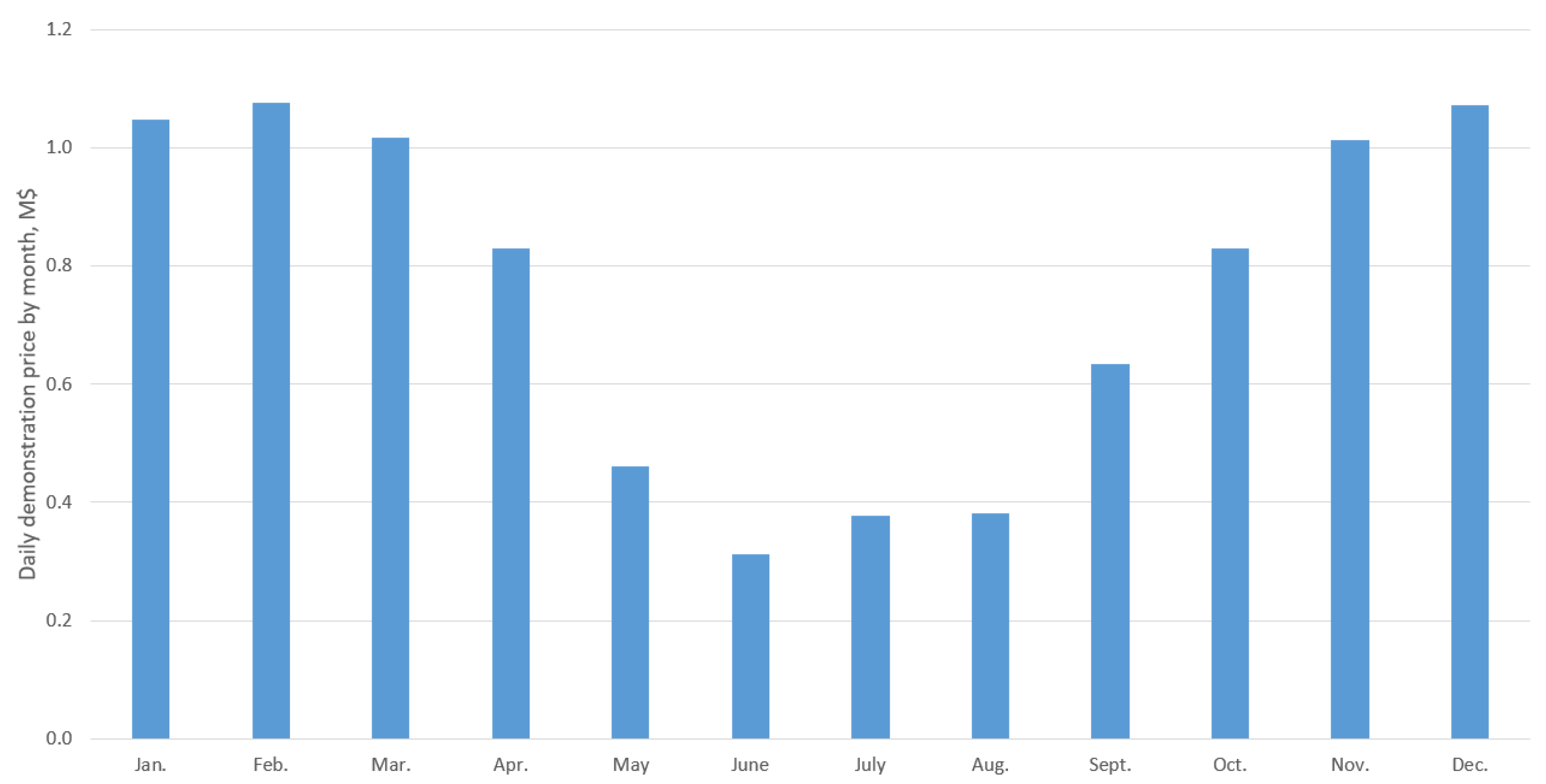
Let us estimate the daily mission revenue using the proposed coverage model and optimizing ground track for different initial conditions such as initial orbit epoch and footprint area presented in Table 1. First of all, the dependence of the mission revenue on the initial orbit epoch or the mission start date is to be determined. As stated in Section 6.2, the demonstration price depends on the time of the year. Therefore, we shall optimize the ground track for the mission performed in different months. Taking into account that the optimization process is time consuming, we consider only one case for the satellite footprint area corresponding to the mid value of pixel magnitude yielding km. The simulation allows finding the appropriate time for the space advertising missions.
Figure 20 shows the distribution of the daily price of image demonstrations by month. It can be seen that the space advertising is most profitable in winter. Therefore, the image demonstration mission in December is considered that corresponds to the initial condition presented in Table 3.
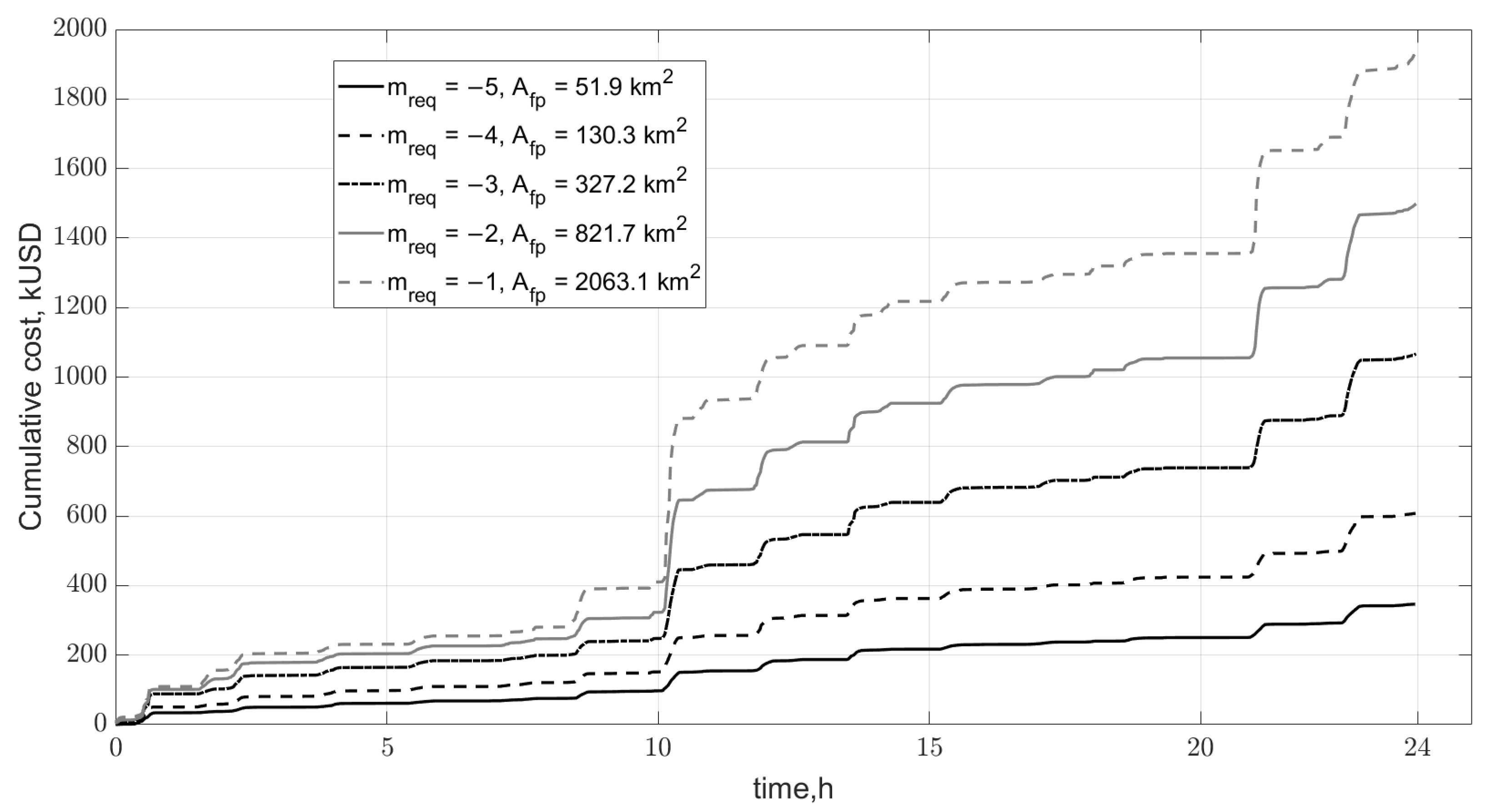
Let us find the dependence of the daily mission revenue on different footprint areas . For this purpose, the mission revenue is optimized according to (31) for the footprint area from Table 1. Figure 21 demonstrates cumulative price curves for demonstrations performed with reflectors of different half beam angles defined in Table 1. Table 4 represents the optimization results.
The animation [34] demonstrates the Earth coverage within the demonstration mission.
7. Results
Assessment of the mission expenses requires calculating the cost of all components including technical support and development. This analysis is carried out in accordance with [35]. The main costs are classified into three major segments: production, technical support, and launch.
The production segment includes spacecraft and payload manufacture. A 12U-cubesat is selected as the spacecraft bus. Payload components are assumed to be analogous to those of the SCOUT spacecraft [36] because of similar solar sail and propulsion subsystem requirements. By rough estimates, such costs add up to about 75% of the total cost of the mission. For instance, the cost of production of the single example of a such spacecraft amounts to approximately $1.765 million. For the manufacture of satellites in the amount of N = 50 units, the cost of a single device can be significantly reduced in mass production. The special technique to account for productivity improvements as a larger number of units is produced named the learning curve is used [35]. The total production cost for N devices is determined as:
where —cost of single satellite, L—the learning curve factor, S—the learning curve slope in percent represented the percentage reduction in cumulative average cost when the number of production units is doubled. S is assumed to be 90% (as recommended in [35]) for 50 units. In these terms, L = 27.6, which means an average price reduction of one satellite by 45%. Thus, the total cost of production is estimated as $ 48.7 million.
The segment of technical support included test and verification, ground, orbital support, and program engineering. This expenditure is calculated by taking into account the cost of all groups of spacecrafts and makes up 17% of the total cost or $ 11.5 million.
Finally, the cost of launch is taken in consideration. The price of putting into orbit 1 tonne is approximately 4.5 M$ according to data reported in [37]. By this means, the total cost of the mission is estimated by the following expression:
The estimate of the resulting cost of the mission is $ 65 million.
To assess the feasibility of a space advertising campaign, the payback period is found according to (34) and compared with the formation lifetime calculated in Section 5.4 using formula (23).
The results are illustrated in Figure 22. The feasibility of the mission significantly depends on the satellite footprint area yielding a different daily mission revenue P as well as on the formation lifetime which is set by the formation satellite parameters and varies depending on the number of reconfigurations. It is assumed that the mission is economically feasible if its lifetime is greater than the payback period .
It can be seen that the formation with satellites equipped with flat reflectors is not economically feasible because it requires the lifetime of about a half of a year which is not reachable for the considered orbital configurations and spacecraft parameters. A greater satellite footprint area allows increasing mission’s daily revenue and hence decreasing payback period, thus making the mission economically feasible. However, the greater the footprint area, the dimmer is the demonstrated image. For example, a mission demonstrating images with magnitude of individual pixels has the payback period of 33.7 days, while a formation operating for 91.5 days (for = 2 kg) can perform 24 image demonstrations within the lifetime, meaning 24 potential contractors for the mission with a net income of about 111.6 million USD.
8. Conclusions and Discussion
The study outlines the framework for satellite formation-flying mission design and analysis. In particular, the framework is used for assessing technical and economical feasibility of space advertising performed with the aid of formation of solar sail-equipped small satellites.
An unrealistic idea as it may first seem, space advertising turns out to have a potential for commercial viability. Our analysis indicates that the two key factors affecting the effectiveness of the mission are satellite footprint area and formation lifetime. The former requires a diffusive solar reflector with a scattering angle greater than the angular size of the Sun. It follows from our simulations that technically feasible solar reflectors of the size that has already been used in CubeSat missions are sufficient for space advertising missions to be economically viable. Obviously, any future advances in solar sailing technologies can enhance the mission performance. As for the mission lifetime, in this work, we confined ourselves to a crude estimate of the upper-bound lifetime value. However, better precision can be obtained using multi-step assignment problem solutions with the aid of deep q-learning or other combinatorial optimization approaches. The estimates of reconfiguration numbers we operate with are reliable enough to give a sense of what can be achieved within one mission.
Lastly, we feel obliged to comment on a frequent objection to a space advertising mission, which is the sky pollution that it may cause, thus thwarting the astronomical observations. Let us recall that the proposed target orbit is aligned near to terminator plane. It allows performing demonstrations only at about the time of sunrise or sunset due the orbit geometry, thus excluding night demonstrations. In addition, numerical analysis of Earth coverage demonstrated that the best strategy for economic feasibility of the system is to perform demonstrations at megalopolises with big population and high CPM. The cities typically have permanent light pollution and are not considered as locations for observatories for which the image demonstration can be harmful.
Author Contributions
Conceptualization, S.B. and D.P.; methodology, S.B.; software, S.B.; validation, S.B., D.P. and G.B.; writing—original draft preparation, S.B.; writing—review and editing, D.P.; visualization, S.B.; supervision, D.P.; funding acquisition, S.B. All authors have read and agreed to the published version of the manuscript.
Funding
The presented study was funded by the Russian Foundation for Basic Research (RFBR), project number 20-31-90115.
Institutional Review Board Statement
Not applicable.
Informed Consent Statement
Not applicable.
Data Availability Statement
Data derived from public domain resources. URLs are provided in the list of references.
Acknowledgments
The authors are grateful to Rory Lipkis for fruitful discussions which contributed to the study.
Conflicts of Interest
The authors declare no conflict of interest. The funders had no role in the design of the study; in the collection, analyses, or interpretation of data; in the writing of the manuscript, or in the decision to publish the results.
Appendix A. Linear Quadratic Regulator Gain Matrix K for Satellite Formation Reconfiguration
Appendix B. Linear Quadratic Regulator Gain Matrix K for Satellite Formation Maintenance
References
- The Wall Street Journal. Pizza Hut Chooses to Embrace A Pie-in-the-Sky Ad Strategy. 1999. Available online: https://www.wsj.com/articles/SB938647339433252633 (accessed on 29 June 2022).
- Wilson, M. Advertising in Space—Spaceflight & Aerospace Industry Marketing. 2018. Available online: https://martinwilson.me/advertising-in-outer-space (accessed on 29 June 2022).
- Nathaniel Lee, R. Elon Musk Sent a 100K $ Tesla Roadster to Space a Year Ago. It has Now Traveled Farther than Any Other Car in History. 2019. Available online: https://www.businessinsider.com/elon-musk-tesla-roadster-space-spacex-orbit-2019-2 (accessed on 29 June 2022).
- Avant Space. Orbital Display. 2018. Available online: https://avantspace.com/en (accessed on 29 June 2022).
- Chow, D. This Russian Startup Wants to Put Huge Ads in Space. Not Everyone is on Board with the Idea. 2019. Available online: https://www.nbcnews.com/mach/science/startup-wants-put-huge-ads-space-not-every-one-board-idea-ncna960296 (accessed on 29 June 2022).
- REUTERS, F. Europe Plans to Orbit Ring of Light to Hail Eiffel Tower. 1986. Available online: https://www.latimes.com/archives/la-xpm-1986-11-24-mn-12955-story.html (accessed on 29 June 2022).
- Rossen, J. Ad Astra: The Time Earth Almost Got a Space Billboard. 2018. Available online: https://www.mentalfloss.com/article/557485/when-earth-almost-got-space-billboard (accessed on 19 July 2021).
- Biktimirov, S.; Ivanov, D.; Pritykin, D. A satellite formation to display pixel images from the sky: Mission design and control algorithms. Adv. Space Res. 2022, 69, 4026–4044. [Google Scholar] [CrossRef]
- Kishida, Y. Changes in Light Intensity at Twilight and Estimation of the Biological Photoperiod. Jpn. Agric. Res. Q. 1989, 22, 247–252. [Google Scholar]
- Ivanov, D.; Biktimirov, S.; Chernov, K.; Kharlan, A.; Monakhova, U.; Pritykin, D. Writing with Sunlight: Cubesat Formation Control Using Aerodynamic Forces. In Proceedings of the International Astronautical Congress, IAC, Washington, DC, USA, 21–25 October 2019. [Google Scholar]
- Vallado, D.A. Fundamentals of Astrodynamics and Applications; Springer Science & Business Media: Berlin/Heidelberg, Germany, 2001; Volume 12. [Google Scholar]
- Cox, A.N. (Ed.) Allen’s Astrophysical Quantities, 4th ed.; AIP Press: New York, NY, USA; Springer: New York, NY, USA, 2000; p. 719. [Google Scholar]
- Canady, J.E.; Allen, J.L. NASA Technical Paper 2065: Illumination from Space with Orbiting Solar-Reflector Spacecraft; Technical Report; Langley Research Center: Hampton, VA, USA, 1982. [Google Scholar]
- Biddy, C.; Svitek, T. LightSail-1 Solar Sail Design and Qualification. In Proceedings of the 41st Aerospace Mechanisms Symposium, Pasadena, CA, USA, 16–18 May 2012. [Google Scholar]
- Palla, C.; Kingston, J.; Hobbs, S. Development of Commercial Drag-Augmentation Systems for Small Satellites. In Proceedings of the 7th European Conference on Space Debris, Darmstadt, Germany, 18–21 April 2017; ESA Space Debris Office: Darmstadt, Germany, 2017. [Google Scholar]
- Spencer, D.A.; Johnson, L.; Long, A.C. Solar sailing technology challenges. Aerosp. Sci. Technol. 2019, 93, 105276. [Google Scholar] [CrossRef]
- Wiltshire, R.; Clohessy, W. Terminal Guidance System for Satellite Rendezvous. J. Aerosp. Sci. 1960, 27, 653–658. [Google Scholar] [CrossRef]
- Alfriend, K.T.; Vadali, S.R.; Gurfil, P.; How, J.P.; Breger, L. Spacecraft Formation Flying: Dynamics, Control and Navigation; Elsevier: Amsterdam, The Netherlands, 2009; Volume 2. [Google Scholar]
- D’Amico, S.; Montenbruck, O. Differential GPS: An Enabling Technology for Formation Flying Satellites. In Proceedings of the Small Satellite Missions for Earth Observation; Sandau, R., Roeser, H.P., Valenzuela, A., Eds.; Springer: Berlin/Heidelberg, Germany, 2010; pp. 457–465. [Google Scholar]
- Arlas, J.; Spangelo, S. GPS Results for the Radio Aurora Explorer II CubeSat Mission. In Proceedings of the 51st AIAA Aerospace Sciences Meeting including the New Horizons Forum and Aerospace Exposition, Grapevine, TX, USA, 7–10 January 2013. [Google Scholar] [CrossRef] [Green Version]
- Bonin, G.; Roth, N.; Armitage, S.; Newman, J.; Risi, B.; Zee, R.E. CanX-4 and CanX-5 Precision Formation Flight: Mission Accomplished! In Proceedings of the 29th Annual AIAA/USU Conference on Small Satellites, Logan, UT, USA, 8–13 August 2015. [Google Scholar]
- Giralo, V.; D’Amico, S. Distributed multi-GNSS timing and localization for nanosatellites. NAVIGATION 2019, 66, 729–746. [Google Scholar] [CrossRef]
- Blank, J.; Deb, K. pymoo: Multi-Objective Optimization in Python. IEEE Access 2020, 8, 89497–89509. [Google Scholar] [CrossRef]
- Duff, I.S.; Koster, J. On Algorithms For Permuting Large Entries to the Diagonal of a Sparse Matrix. SIAM J. Matrix Anal. Appl. 2001, 22, 973–996. [Google Scholar] [CrossRef] [Green Version]
- Dawn Aerospace. B1 Thruster. Available online: https://www.dawnaerospace.com/products/satdriveb1 (accessed on 29 June 2022).
- European Commission. Atlas of the Human Planet 2018—A World of Cities; EUR 29497 EN; European Commission, Joint Research Centre: Luxembourg, 2018; ISBN 978-92-79-98185-2. [Google Scholar] [CrossRef]
- Guttmann, A. Year-on-Year Change in CPM of Standard Billboard Advertising Worldwid. 2018. Available online: https://www.statista.com/statistics/868305/change-cost-per-mille-billboard-advertising (accessed on 29 June 2022).
- WARC. Global Ad Market Will Take Years to Recover from COVID-19. 2020. Available online: https://www.warc.com/newsandopinion/news/global-ad-market-will-take-years-to-recover-from-covid-19/44417 (accessed on 29 June 2022).
- Salnicoff, A. Over the Road Billboards and Banners Effectiveness. Pract. Mark. 2015, 1, 33–42. [Google Scholar]
- Platnick, S.; Ackerman, S.; King, M.; Meyer, K.; Penzel, W.; Holz, R.; Baum, B.; Yang, P. MODIS Atmosphere L2 Cloud Product (06_L2). 2021. Available online: https://doi.org/10.5067/MODIS/MOD06_L2.006 (accessed on 29 June 2022).
- Salnicoff, A. How Pedestrians Pay Attention to Small size Outdoor Advertising. Pract. Mark. 2014, 2, 17–27. [Google Scholar]
- United Nations Population Division of the Department of Economic and Social Affairs. Data on Age and Gender Distribution of Population by Country. 2019. Available online: https://population.un.org/wpp (accessed on 29 June 2022).
- Lagarias, J.C.; Reeds, J.A.; Wright, M.H.; Wright, P.E. Convergence properties of the Nelder—Mead simplex method in low dimensions. SIAM J. Optim. 1998, 9, 112–147. [Google Scholar] [CrossRef] [Green Version]
- Biktimirov, S.; Belyj, G.; Pritykin, D. Animation of Earth Coverage. Available online: https://disk.yandex.ru/d/VPeuH-H8ptsLyw (accessed on 29 June 2022).
- Wertz, J.R.; Larson, W.J. Space Mission Analysis and Design, 3rd ed.; Microcosm Press: Torrance, CA, USA; Kluwer Academic: Dordrecht, The Netherlands, 1999. [Google Scholar]
- ESA Earth Observation Portal. NEA Scout (Near Earth Asteroid Scout) CubeSat Mission. 2019. Available online: https://directory.eoportal.org/web/eoportal/satellite-missions/n/nea-scout (accessed on 29 June 2022).
- Launch Cost of Satellites. 2021. Available online: https://spaceflight.com/pricing (accessed on 29 June 2022).
Figure 1.
Reference frames [8].
Figure 1.
Reference frames [8].

Figure 2.
Orbit geometry [8].
Figure 2.
Orbit geometry [8].

Figure 3.
Reflector sizing geometry.

Figure 4.
Reflector parameters.

Figure 5.
Demonstration campaign images.

Figure 6.
LQR gains optimization.

Figure 7.
Satellite dynamics and control at deployment to the farthest reference trajectory.

Figure 8.
(a) Reconfiguration cost , (b) image’s relative orientation for .

Figure 9.
Fuel consumption estimates for satellite formation reconfiguration and maintenance.

Figure 10.
Fuel consumption estimates.

Figure 11.
Coverage geometry.

Figure 12.
Coverage visualization.

Figure 13.
Average CPM in world countries in 2018.

Figure 14.
The seasonal coefficient.

Figure 15.
The cloud interference coefficient.

Figure 16.
OTS discounting coefficients comparison.

Figure 17.
Price demonstration map of the world.

Figure 18.
Demonstration price distribution over the Earth regions.

Figure 19.
Ground track for different initial conditions.

Figure 20.
Daily price distribution by month.

Figure 21.
Cumulative demonstrations price.

Figure 22.
Space advertising system performance analysis.


Table 1.
Mission Parameters.
| , arcmin | , km | |
|---|---|---|
| −5 | 15.6 | 51.9 |
| −4 | 24.7 | 130.3 |
| −3 | 39.2 | 327.2 |
| −2 | 62.1 | 821.7 |
| −1 | 98.4 | 2063.4 |
Table 2.
Simulation parameters.
| Paramater | Value | Units |
|---|---|---|
| Target orbit | ||
| Altitude | 895.45 | km |
| Inclination | 98.98 | deg |
| Satellite parameters | ||
| Mass | 18 | kg |
| [25] | 0.4 | N |
| [25] | 285 | s |
| Admissible control errors at reconfiguration | ||
| 50 | m | |
| 0.5 | m/s | |
| Admissible control errors at maintenance | ||
| 1 | m | |
| 0.1 | m/s | |
Table 3.
Target orbit parameters.
| Epoch (UTC) | |||||
|---|---|---|---|---|---|
| 22/12/2022, 00:00:00 | 895.45 | 0 | 0 |
Table 4.
Coverage optimization results.
| , km | m | , deg | P, mln USD | |
|---|---|---|---|---|
| 51.9 | −5 | 35.20 | 491 | 0.35 |
| 130.3 | −4 | 39.96 | 498 | 0.61 |
| 327.2 | −3 | 37.31 | 493 | 1.07 |
| 821.7 | −2 | 37.31 | 493 | 1.50 |
| 2063.4 | −1 | 37.31 | 493 | 1.93 |
Publisher’s Note: MDPI stays neutral with regard to jurisdictional claims in published maps and institutional affiliations. |
© 2022 by the authors. Licensee MDPI, Basel, Switzerland. This article is an open access article distributed under the terms and conditions of the Creative Commons Attribution (CC BY) license (https://creativecommons.org/licenses/by/4.0/).
Share and Cite
MDPI and ACS Style
Biktimirov, S.; Belyj, G.; Pritykin, D. Satellite Formation Flying for Space Advertising: From Technically Feasible to Economically Viable. Aerospace 2022, 9, 419. https://doi.org/10.3390/aerospace9080419
AMA Style
Biktimirov S, Belyj G, Pritykin D. Satellite Formation Flying for Space Advertising: From Technically Feasible to Economically Viable. Aerospace. 2022; 9(8):419. https://doi.org/10.3390/aerospace9080419
Chicago/Turabian StyleBiktimirov, Shamil, Gleb Belyj, and Dmitry Pritykin. 2022. "Satellite Formation Flying for Space Advertising: From Technically Feasible to Economically Viable" Aerospace 9, no. 8: 419. https://doi.org/10.3390/aerospace9080419
Note that from the first issue of 2016, this journal uses article numbers instead of page numbers. See further details here.